Building a Work Zone Digital Twin

Work zone compliance today is measured one frame at a time. A field inspector walks the site, takes photos, fills out a checklist. That approach is slow, inconsistent, and it produces no spatial model of the work zone as a physical object in three-dimensional space.

We wanted to change that. The question we set out to answer was whether a single dashcam video pass, combined with the GPS telemetry a crew vehicle is already recording, could produce calibrated 3D measurements of work zone assets accurate enough to be operationally useful. Taper length. Channelizer spacing. Sign-to-taper distance. The numbers that determine whether a work zone is MUTCD-compliant.

After building a twelve-stage offline pipeline and validating it against ground truth measurements, the answer is yes, with important caveats about what the data needs to look like and where the pipeline can fail.

This post walks through how we built it and what we learned.

Structure from Motion on a Budget

The technique underlying the pipeline is Structure from Motion, or SfM. It is a well-established approach in photogrammetry that reconstructs 3D geometry from a sequence of overlapping 2D images. What makes this interesting for work zones is that a dashcam driving through a site is already producing exactly the kind of image sequence SfM needs. A continuous set of overlapping frames from a moving camera, with known approximate positions from GPS.

The challenge is that raw SfM gives you geometry in an arbitrary scale. The 3D point cloud it produces is internally consistent, but the units are meaningless until you anchor them to real-world distance. And GPS alone is not precise enough to do that anchoring directly, not at the sub-meter accuracy you need to measure channelizer spacing.

So the pipeline has two distinct halves. The reconstruction half builds the 3D model. The metric half grounds it in the physical world.

The Twelve-Stage Pipeline

The pipeline moves through five groups of stages: ingest, reconstruct, annotate, measure, and output. Each stage emits a QC JSON artifact so any failure is loud and traceable.

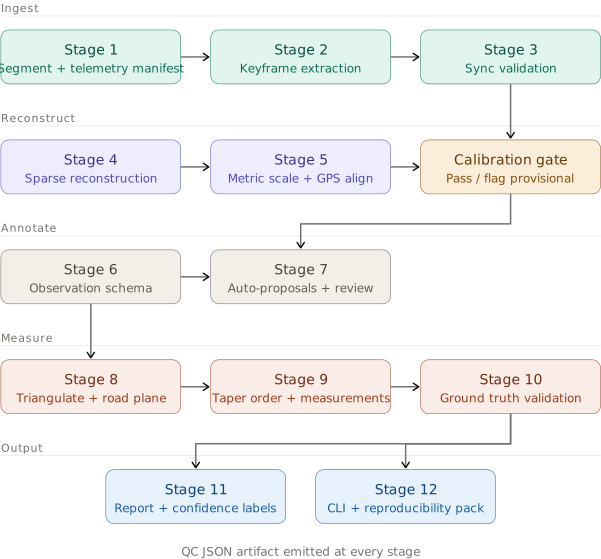
Stage 1 - Segment and Telemetry Manifest

Everything starts with a canonical input format. The pipeline ingests a single campaign segment, a video file and a telemetry manifest in CSV or JSON with per-frame timestamps, GPS coordinates, vehicle speed, and heading. Getting this right at the front end matters because every downstream stage depends on the telemetry-to-frame index being correct. The manifest validator rejects inputs with timestamp gaps, coordinate jumps, or missing fields rather than silently propagating bad data.

Stage 2 - Keyframe Extraction and Frame Index

Running SfM on every frame is wasteful and introduces reconstruction instability from near-identical consecutive images. The keyframe extractor subsamples the video at a target overlap ratio, typically 70 to 80 percent overlap between consecutive keyframes, using both visual distinctiveness and GPS displacement as selection criteria. Each extracted keyframe gets a record in the frame and telemetry index, including frame number, timestamp, GPS position, and heading. This index becomes the lookup table for every subsequent stage.

Stage 3 - Synchronization Validation and Window Selection

Video and telemetry clocks drift. A camera and a GPS logger running independently will accumulate offset over a recording session, and even a one-second offset at 60 km/h moves the camera 17 meters from where the telemetry says it was. The sync validation stage cross-correlates visual motion magnitude with GPS-derived speed to estimate and correct clock offset. If the estimated offset exceeds a configurable threshold, the stage fails the segment rather than proceeding with misaligned data. The output is a validated reconstruction window covering the span of frames and telemetry the pipeline will operate on.

Stage 4 - Sparse Reconstruction

With a validated keyframe set, the pipeline runs COLMAP’s incremental SfM to produce a sparse 3D reconstruction, a set of camera poses and a sparse point cloud. The output at this stage is in arbitrary scale. The geometry is correct in shape and proportion, but the unit of measurement is undefined. Camera poses are exported as rotation matrices and translation vectors for the metric recovery stage.

Stage 5 - Metric Scale Recovery and GPS Alignment

This is where the reconstruction gets grounded. The pipeline fits a similarity transform between the SfM camera trajectory and the GPS-derived camera positions, solving for scale, rotation, and translation simultaneously. The scale factor converts the arbitrary-unit SfM output into meters. GPS alignment orients the model in East-North-Up coordinates.

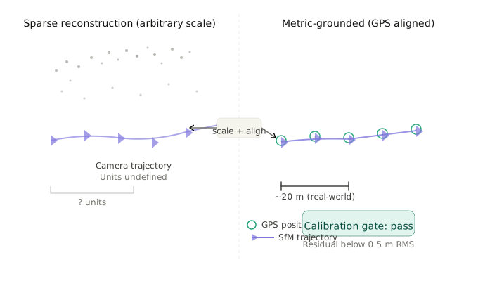
The calibration gate is the most important safeguard in the pipeline. If the residual between the GPS-aligned trajectory and the SfM trajectory exceeds 0.5 meters RMS, the segment is flagged and measurements are labeled provisional. In practice, this gate catches segments where GPS signal was degraded or where the reconstruction window was too short to constrain scale reliably.

Stage 6 - Observation Schema and Annotation Tool

At this point the pipeline has a calibrated 3D model but no semantic content. It does not know where the cones are, where the signs are, or where the taper begins and ends. The observation schema defines the data structure for work zone asset annotations, covering asset type, 2D pixel coordinates in one or more keyframes, confidence score, and provenance as either manual or auto-proposed.

The annotation tool is deliberately minimal. It is a lightweight viewer that displays keyframes with the sparse point cloud projected as an overlay and lets a reviewer click to place observations. Keeping the tool simple was a deliberate choice because the goal for this POC was to validate the pipeline’s geometric accuracy, not to build production annotation tooling.

Stage 7 - Auto-Proposal Import and Reviewer Assist

Manual annotation does not scale. The auto-proposal stage runs a detection model fine-tuned on work zone assets over the keyframe set and imports detections as draft observations in the same schema as manual annotations. The reviewer assist flow highlights high-confidence auto-proposals for quick confirmation and flags low-confidence proposals for closer review. The schema makes manual and automatic observations interchangeable downstream. The triangulation stage does not care how an observation was produced.

Stage 8 - Asset Triangulation and Road Plane Fitting

With observations confirmed across multiple keyframes, the pipeline triangulates each asset’s 3D base point using the calibrated camera poses. For channelizers like cones and drums, the base point is the ground contact. For signs, it is the post base. A road plane is fit to the ensemble of channelizer base points using RANSAC to suppress outliers. All asset positions are projected onto this plane for measurement, which removes the effect of road grade and cross-slope on distance calculations.

Stage 9 - Taper Ordering and Measurement Computation

Assets are ordered along the taper using their projected positions on the road plane. From the ordered asset sequence, the pipeline computes three primary measurements. Channelizer taper length is the distance from the first to last channelizer along the taper centerline. Mean spacing is the average longitudinal distance between consecutive channelizers. Sign-to-taper distance is the distance from each sign’s base point to the first channelizer in the taper, projected onto the road centerline.

Each measurement gets a confidence label derived from the reconstruction residual, observation count, and RANSAC inlier ratio.

Stage 10 - Ground Truth Validation

The pipeline includes a validation stage that ingests field-measured ground truth from manual tape measurements or survey-grade GPS and computes per-measurement error. For the POC validation campaign, we measured several work zone segments across active construction sites. All measurements fell within the MUTCD tolerance bands for the corresponding speed environments.

The failure-mode catalog, generated from segments where the calibration gate triggered, points consistently to two root causes. GPS multipath in urban canyon environments is one. Reconstruction windows shorter than approximately 150 meters are the other, because they do not provide enough baseline for reliable scale recovery.

Stage 11 - Report Generation and Confidence Labels

Every pipeline run produces a QC JSON artifact at each stage. The final report aggregates these into a human-readable summary with measurements and confidence labels, a reconstruction quality assessment, and the failure-mode catalog for any segments that did not pass the calibration gate. The report is designed to be auditable so that every number traces back to the observations and camera poses that produced it.

Stage 12 - CLI and Reproducibility Pack

The pipeline runs end-to-end from a single CLI invocation. The reproducibility pack is a zip archive containing the input segment, the keyframe set, the COLMAP workspace, all intermediate artifacts, and the final report. Any stage can be re-run in isolation by pointing the CLI at the appropriate intermediate artifact. Opaque binary state makes debugging impossible, and debugging is most of the work in a POC, so we designed the whole thing to stay inspectable.

What This Enables

The immediate application is compliance measurement at scale. A crew vehicle equipped with a dashcam and a standard GPS logger, equipment most agencies and contractors already have, can drive a work zone and produce calibrated measurements of taper length, channelizer spacing, and sign placement without any manual tape measuring. The pipeline runs offline, produces auditable artifacts, and fails loudly when its inputs are not good enough to trust the outputs.

The longer-term implication is more significant. A calibrated 3D model of a work zone opens up comparison workflows that do not exist today. You can compare a work zone’s actual geometry to its design intent. You can track how a work zone changes over the life of a project, whether channelizer spacing degrades after a weekend, whether signs get relocated, whether the taper shortens as crews push the closure forward. None of that is possible with the current state of the art, which is a collection of flat photos with no spatial relationship to each other.

Current Limitations

This is a POC, not a production service, and the limitations are worth being explicit about. Scale recovery degrades in GPS multipath environments and we are evaluating IMU fusion as a fallback. Reconstruction windows under 150 m do not reliably constrain scale, which means long tapers and complex work zones are better candidates than short closures. The auto-proposal model was trained on a limited set of channelizer types, so unusual device configurations still require manual annotation. And any segment that triggers the calibration gate produces measurements labeled provisional, meaning they are geometrically consistent but may carry metric error above the validation thresholds.

What’s Next

We are extending the pipeline in two directions. First is IMU integration to improve scale recovery in GPS-degraded environments. Second is multi-pass comparison to detect work zone changes between inspection runs, which is the foundation for longitudinal compliance monitoring.

The core insight from this work is that the data agencies need already exists. Crews are already driving through work zones in vehicles with cameras and GPS. The pipeline we have built shows that this data, processed correctly, can produce measurements precise enough for compliance without any additional hardware investment.